Dust Attenuation and Emission#
A fundamental assumption of our normal galaxy (i.e., non AGN) modeling in Lightning is energy balance: the optical power from starlight attenuated by ISM dust is re-radiated in the infrared. As such we present the dust attenuation and emission models side by side here.
Imports#
[1]:
import numpy as np
from scipy.integrate import trapz

from lightning import Lightning
from lightning.attenuation import CalzettiAtten, ModifiedCalzettiAtten, SMC
from lightning.dust import Graybody, DL07Dust

import matplotlib.pyplot as plt
import matplotlib as mpl
plt.style.use('lightning.plots.style.lightning-serif')
%matplotlib inline
Attenuation#
plightning currently contains three attenuation options: Calzetti+(2000), “Modified Calzetti” (Noll+2009, including variable UV slope and a 2175 Å bump), and the SMC attenuation curve (Gordon+2003). Adding tabulated attenuation curves is pretty trivial (see lightning.dust.TabulatedAtten; the SMC curve is an instance of this class). The Doore+(2021) inclination-dependent attenuation curve is coming soon, pending some more testing of computational enhancements I implemented that might not
actually be improvements.
[2]:
wave = np.logspace(np.log10(0.0912),
                   np.log10(5),
                   200)

calz = CalzettiAtten(wave)
modcalz = ModifiedCalzettiAtten(wave)
smc = SMC(wave)

calz.print_params(verbose=True)
modcalz.print_params(verbose=True)
smc.print_params(verbose=True)
============================
Calzetti
============================
     Parameter  Lo  Hi                      Description
-------------- --- --- --------------------------------
calz_tauV_diff 0.0 inf Optical depth of the diffuse ISM

Total parameters: 1

============================
Modified-Calzetti
============================
      Parameter   Lo                 Hi                                                                                Description
--------------- ---- ------------------ ------------------------------------------------------------------------------------------
mcalz_tauV_diff  0.0                inf                                                           Optical depth of the diffuse ISM
    mcalz_delta -inf 0.4473684210526316 Deviation from the Calzetti+2000 UV power law slope (Upper limit set by requiring Eb >= 0)
  mcalz_tauV_BC  0.0                inf                                   Optical depth of the birth cloud in star forming regions

Total parameters: 3

============================
smc
============================
    Parameter  Lo       Hi                      Description
------------- --- -------- --------------------------------
smc_tauV_diff 0.0 100000.0 Optical depth of the diffuse ISM

Total parameters: 1
SMC and Calzetti#
[3]:
fig, axs = plt.subplots(1,3, figsize=(12,4))
plt.subplots_adjust(wspace=0.3)

tauV_arr = np.linspace(0, 1.5, 6).reshape(-1, 1)
Nmod = len(tauV_arr)

cm_calz = mpl.colormaps['Oranges']
colors_calz = cm_calz(np.linspace(0.2, 0.9, Nmod))

cm_smc = mpl.colormaps['Greens']
colors_smc = cm_smc(np.linspace(0.2, 0.9, Nmod))

calz_models = calz.evaluate(tauV_arr)
smc_models = smc.evaluate(tauV_arr)

for i in np.arange(Nmod):
    axs[0].plot(wave, calz_models[i,:], color=colors_calz[i])
    axs[1].plot(wave, smc_models[i,:], color=colors_smc[i])
    axs[2].plot(wave, calz_models[i,:], color=colors_calz[i])
    axs[2].plot(wave, smc_models[i,:], color=colors_smc[i])

axs[0].set_xscale('log')
axs[0].set_yscale('log')
#axs[0].set_ylim(2e6, 1e11)

axs[0].set_xlabel(r'Rest-Frame Wavelength [$\rm \mu m$]')
axs[0].set_ylabel(r'$e^{- \tau}$')
axs[0].set_title('Calzetti')

axs[1].set_xscale('log')
axs[1].set_yscale('log')

axs[1].set_xlabel(r'Rest-Frame Wavelength [$\rm \mu m$]')
axs[1].set_ylabel(r'$e^{- \tau}$')
axs[1].set_title('SMC')

axs[2].set_xscale('log')
axs[2].set_yscale('log')

axs[2].set_xlabel(r'Rest-Frame Wavelength [$\rm \mu m$]')
axs[2].set_ylabel(r'$e^{- \tau}$')
axs[2].set_title('Both')
[3]:
Text(0.5, 1.0, 'Both')
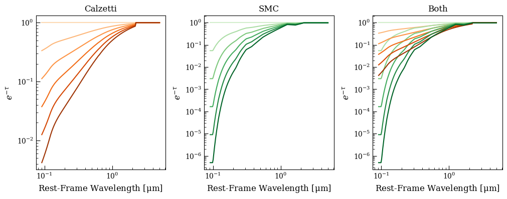
The SMC curve is steeper at UV wavelengths for the same \(\tau_V\). It’s used as the default curve for the AGN polar dust model.
Modified Calzetti#
The main parameters here are the \(V-\)band optical depth (as above) and \(\delta\) the deviation of the UV slope from the Calzetti value. The model also ostensibly allows for extra attenuation for young stars that have not yet blown away their birth cloud (\(\tau_{V, \rm BC}\)) but this is not currently implemented, so that parameter doesn’t do anything. Working on coming up with a solution I like for flexibly allowing differential attenuation based on stellar age (this is also an issue that affects the Doore+2021 model).
[4]:
fig, axs = plt.subplots(figsize=(4,4))
plt.subplots_adjust(wspace=0.3)

param_arr = np.array([[0.1, 0.4, 0.0],
                      [0.1, 0.2, 0.0],
                      [0.1, 0.0, 0.0],
                      [0.1, -0.2, 0.0],
                      [0.1, -0.4, 0.0]])

Nmod = param_arr.shape[0]

cm_calz = mpl.colormaps['Oranges']
color_calz = cm_calz(0.5)

cm_modcalz = mpl.colormaps['Greens']
colors_modcalz = cm_smc(np.linspace(0.2, 0.9, Nmod))

calz_models = calz.evaluate(param_arr[:,0])
modcalz_models = modcalz.evaluate(param_arr)

axs.plot(wave, calz_models[0,:], color=color_calz)

for i in np.arange(Nmod):
    axs.plot(wave, modcalz_models[i,:], color=colors_modcalz[i], label=r'$\delta = %.1f$' % (param_arr[i,1]))

axs.set_xscale('log')
axs.set_yscale('log')

axs.set_xlabel(r'Rest-Frame Wavelength [$\rm \mu m$]')
axs.set_ylabel(r'$e^{- \tau}$')
axs.legend(loc='lower right')
[4]:
<matplotlib.legend.Legend at 0x3218ba910>
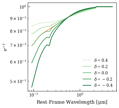
The modified Calzetti model is in green, where lighter \(\rightarrow\) darker colors indicate \(\delta\) changing from positive to negative. The strength of the 2175 Å feature is tied to the UV slope parameter, \(\delta\). Note that the modified Calzetti model is not exactly equal to the Calzetti model with the same \(\tau_V\) when \(\delta = 0\), due to the presence of the 2175 Å absorption feature.
Emission Models#
[5]:
wave_grid = np.logspace(np.log10(1),
                        np.log10(1000),
                        200)
filter_labels = ['IRAC_CH1', 'IRAC_CH2', 'IRAC_CH3', 'IRAC_CH4',
                 'MIPS_CH1',
                 'PACS_green', 'PACS_red',
                 'SPIRE_250', 'SPIRE_350', 'SPIRE_500']

redshift = 0.0

dl07 = DL07Dust(filter_labels,
                redshift=redshift,
                wave_grid=wave_grid)
gb = Graybody(filter_labels,
              redshift=redshift,
              wave_grid=wave_grid)

dl07.print_params(verbose=True)
gb.print_params(verbose=True)
============================
DL07-Dust
============================
      Parameter     Lo       Hi                                                             Description
--------------- ------ -------- -----------------------------------------------------------------------
dl07_dust_alpha  -10.0      4.0                  Radiation field intensity distribution power law index
dl07_dust_U_min    0.1     25.0                                       Radiation field minimum intensity
dl07_dust_U_max 1000.0 300000.0                                       Radiation field maximum intensity
dl07_dust_gamma    0.0      1.0 Fraction of dust mass exposed to radiation field intensity distribution
dl07_dust_q_PAH 0.0047   0.0458                            Fraction of dust mass composed of PAH grains

Total parameters: 5

============================
GrayBody-Dust
============================
Parameter   Lo     Hi                      Description
--------- ---- ------ --------------------------------
  gb_lam0 10.0 1000.0 Wavelength of unit optical depth
  gb_beta  0.1    5.0    Optical depth power law index
     gb_T 10.0  100.0                 Dust temperature

Total parameters: 3
Draine and Li (2017)#
The Draine and Li model carries around its own wavelength grid due to some artifact of how the models were constructed in IDL Lightning. I should aee an option to interpolate it to some other grid for consistency with every other model class…
[6]:
fig, axs = plt.subplots(1,3, figsize=(12,4))

var_umin = np.array([[2, 0.1, 3e5, 0.05, 0.02],
                     [2, 1, 3e5, 0.05, 0.02],
                     [2, 5, 3e5, 0.05, 0.02],
                     [2, 10, 3e5, 0.05, 0.02],
                     [2, 25, 3e5, 0.05, 0.02]])

var_gamma = np.array([[2, 1, 3e5, 0.05, 0.02],
                     [2, 1, 3e5, 0.1, 0.02],
                     [2, 1, 3e5, 0.5, 0.02],
                     [2, 1, 3e5, 0.75, 0.02],
                     [2, 1, 3e5, 1.0, 0.02]])

var_qpah = np.array([[2, 1, 3e5, 0.05, 0.0047],
                     [2, 1, 3e5, 0.05, 0.01],
                     [2, 1, 3e5, 0.05, 0.02],
                     [2, 1, 3e5, 0.05, 0.03],
                     [2, 1, 3e5, 0.05, 0.0458]])

mod_var_umin, L_var_umin = dl07.get_model_lnu_hires(var_umin)
Lmod_var_umin, L_var_umin = dl07.get_model_lnu(var_umin)
mod_var_gamma, L_var_gamma = dl07.get_model_lnu_hires(var_gamma)
Lmod_var_gamma, L_var_gamma = dl07.get_model_lnu(var_gamma)
mod_var_qpah, L_var_qpah = dl07.get_model_lnu_hires(var_qpah)
Lmod_var_qpah, L_var_qpah = dl07.get_model_lnu(var_qpah)

Nmod = var_umin.shape[0]

cm_umin = mpl.colormaps['Oranges']
colors_umin = cm_umin(np.linspace(0.2, 0.9, Nmod))

cm_gamma = mpl.colormaps['Greens']
colors_gamma = cm_gamma(np.linspace(0.2, 0.9, Nmod))

cm_qpah = mpl.colormaps['Blues']
colors_qpah = cm_qpah(np.linspace(0.2, 0.9, Nmod))

for i in np.arange(Nmod):

    axs[0].plot(dl07.wave_grid_rest, dl07.nu_grid_rest * mod_var_umin[i,:] / L_var_umin[i], color=colors_umin[i], label=r'$U_{\rm min} = %.1f$' % (var_umin[i,1]))
    axs[0].scatter(dl07.wave_obs, dl07.nu_obs * Lmod_var_umin[i,:] / L_var_umin[i], color=colors_umin[i], marker='D')
    axs[1].plot(dl07.wave_grid_rest, dl07.nu_grid_rest * mod_var_gamma[i,:] / L_var_gamma[i], color=colors_gamma[i], label=r'$\gamma = %.2f$' % (var_gamma[i,3]))
    axs[1].scatter(dl07.wave_obs, dl07.nu_obs * Lmod_var_gamma[i,:] / L_var_gamma[i], color=colors_gamma[i], marker='D')
    axs[2].plot(dl07.wave_grid_rest, dl07.nu_grid_rest * mod_var_qpah[i,:] / L_var_qpah[i], color=colors_qpah[i], label=r'$q_{\rm PAH} = %.4f$' % (var_qpah[i,4]))
    axs[2].scatter(dl07.wave_obs, dl07.nu_obs * Lmod_var_qpah[i,:] / L_var_qpah[i], color=colors_qpah[i], marker='D')

axs[0].set_xscale('log')
axs[0].set_yscale('log')
axs[0].set_xlabel(r'Rest-Frame Wavelength [$\rm \mu m$]')
axs[0].set_ylabel(r'$L_\nu / L_{\rm IR}$ [a.u.]')
axs[0].set_ylim(1e-5, 1)
axs[0].legend(loc='lower left', frameon=True)
#axs[0].set_title(r'$U_{\rm min}=0.1\rightarrow25$')

axs[1].set_xscale('log')
axs[1].set_yscale('log')
axs[1].set_xlabel(r'Rest-Frame Wavelength [$\rm \mu m$]')
axs[1].set_yticklabels([])
axs[1].set_ylim(1e-5, 1)
axs[1].legend(loc='lower left', frameon=True)
#axs[1].set_title(r'$\gamma=0.05\rightarrow1$')

axs[2].set_xscale('log')
axs[2].set_yscale('log')
axs[2].set_xlabel(r'Rest-Frame Wavelength [$\rm \mu m$]')
axs[2].set_yticklabels([])
axs[2].set_ylim(1e-5, 1)
axs[2].legend(loc='lower left', frameon=True)
#axs[2].set_title(r'$q_{\rm PAH}=0.0047\rightarrow0.0458$')
[6]:
<matplotlib.legend.Legend at 0x32189b810>
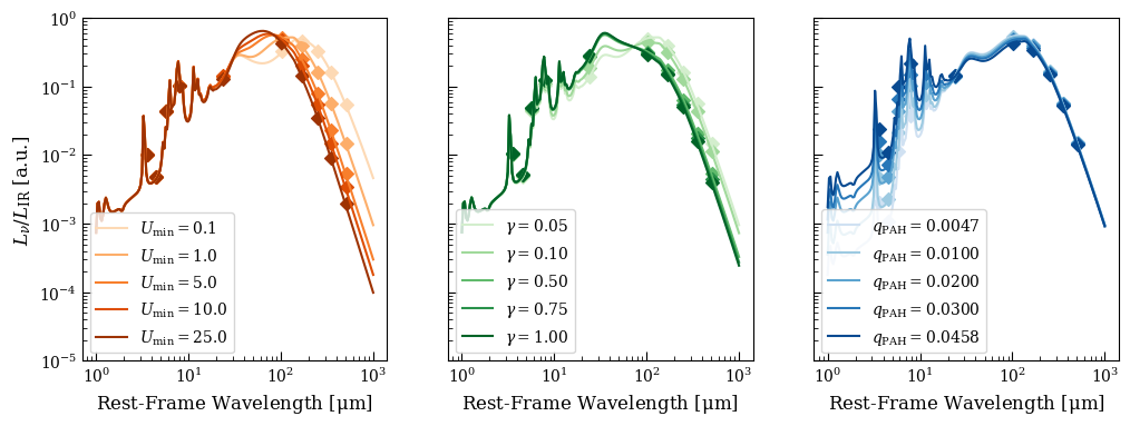
In each of the above plots the changing parameter goes from lighter \(\rightarrow\) darker lines. Note that in practice the normalization of the model is set by the attenuated power from starlight.
Graybody#
This model is currently used in our modeling only to represent the re-emission component of the AGN polar dust model.
[7]:
fig, axs = plt.subplots(1,3, figsize=(12,4))

var_lam0 = np.array([[10, 1, 10],
                     [100, 1, 10],
                     [200, 1, 10],
                     [500, 1, 10],
                     [1000, 1, 10]])

var_beta = np.array([[100, 0.1, 10],
                     [100, 1, 10],
                     [100, 1.5, 10],
                     [100, 2, 10],
                     [100, 5, 10]])

var_temp = np.array([[100, 1, 10],
                     [100, 1, 20],
                     [100, 1, 50],
                     [100, 1, 75],
                     [100, 1, 100]])

mod_var_lam0 = gb.get_model_lnu_hires(var_lam0)
mod_var_beta = gb.get_model_lnu_hires(var_beta)
mod_var_temp = gb.get_model_lnu_hires(var_temp)

Nmod = var_umin.shape[0]

cm_lam0 = mpl.colormaps['Oranges']
colors_lam0 = cm_lam0(np.linspace(0.2, 0.9, Nmod))

cm_beta = mpl.colormaps['Greens']
colors_beta = cm_beta(np.linspace(0.2, 0.9, Nmod))

cm_temp = mpl.colormaps['Blues']
colors_temp = cm_temp(np.linspace(0.2, 0.9, Nmod))

for i in np.arange(Nmod):

    axs[0].plot(gb.wave_grid_rest, gb.nu_grid_rest * mod_var_lam0[i,:], color=colors_lam0[i], label=r'$\lambda_0 = %d$' % (var_lam0[i,0]))
    axs[1].plot(gb.wave_grid_rest, gb.nu_grid_rest * mod_var_beta[i,:], color=colors_beta[i], label=r'$\beta = %.1f$' % (var_beta[i,1]))
    axs[2].plot(gb.wave_grid_rest, gb.nu_grid_rest * mod_var_temp[i,:], color=colors_temp[i], label=r'$T = %d$' % (var_temp[i,2]))

axs[0].set_xscale('log')
axs[0].set_yscale('log')
axs[0].set_xlabel(r'Rest-Frame Wavelength [$\rm \mu m$]')
axs[0].set_ylabel(r'$L_\nu / L_{\rm IR}$ [a.u.]')
axs[0].set_ylim(1e-5, 5)
axs[0].set_xlim(10, 1000)
#axs[0].set_title(r'$\lambda_{0}=10\rightarrow1000~\rm \mu m$')
axs[0].legend(loc='lower left', frameon=True)

axs[1].set_xscale('log')
axs[1].set_yscale('log')
axs[1].set_xlabel(r'Rest-Frame Wavelength [$\rm \mu m$]')
axs[1].set_ylim(1e-5, 5)
axs[1].set_xlim(10, 1000)
#axs[1].set_title(r'$\beta=0.1\rightarrow5$')
axs[1].legend(loc='lower left', frameon=True)


axs[2].set_xscale('log')
axs[2].set_yscale('log')
axs[2].set_xlabel(r'Rest-Frame Wavelength [$\rm \mu m$]')
axs[2].set_ylim(1e-5, 5)
axs[2].set_xlim(10, 1000)
#axs[2].set_title(r'$T=10\rightarrow100~\rm K$')
axs[2].legend(loc='lower left', frameon=True)
/Users/eqm5663/Research/code/plightning/lightning/dust/gray.py:120: RuntimeWarning: overflow encountered in exp
  (np.exp(hcoverk / (wave_g1um[None,:] * T[:,None])) - 1)
[7]:
<matplotlib.legend.Legend at 0x32339dc10>
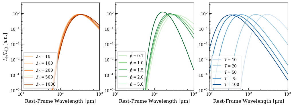
Again, for energy balance the model should be normalized to the total attenuated power.