Stellar Population Model Comparison - NGC 337#
In this notebook we compare the models with the new nebular components from Cloudy simulations to each other and to the PEGASE model stellar populations used in the IDL version of Lightning, fitting all the models to the Dale+(2017) photometry for NGC 337 and comparing the results and derived properties.
Imports#
[1]:
import numpy as np
import h5py
rng = np.random.default_rng()
import astropy.units as u
from astropy.table import Table
from corner import corner
import matplotlib.pyplot as plt
plt.style.use('lightning.plots.style.lightning-serif')
%matplotlib inline

from lightning import Lightning
from lightning.priors import UniformPrior, ConstantPrior
Setup#
We’re defining three different Lightning instances that use the same photometry:
PEGASE model populations from IDL Lightning
PEGASE model populations with Cloudy simulations
BPASS model populations with Cloudy simulations
[9]:
cat = Table.read('../photometry/ngc337_dale17_photometry.fits')

filter_labels = np.array([s.decode().strip() for s in cat['FILTER_LABELS'].data[0]])
fnu_obs = cat['FNU_OBS'].data[0]
fnu_unc = cat['FNU_UNC'].data[0]
dl = cat['LUMIN_DIST'].data[0]

lgh_pg = Lightning(filter_labels,
                   lum_dist=dl,
                   stellar_type='PEGASE',
                   SFH_type='Piecewise-Constant',
                   atten_type='Modified-Calzetti',
                   dust_emission=True,
                   model_unc=0.10,
                   print_setup_time=True)

lgh_pg.flux_obs = fnu_obs * 1e3
lgh_pg.flux_unc = fnu_unc * 1e3

lgh_pg_cl = Lightning(filter_labels,
                      lum_dist=dl,
                      stellar_type='PEGASE-A24',
                      SFH_type='Piecewise-Constant',
                      atten_type='Modified-Calzetti',
                      dust_emission=True,
                      model_unc=0.10,
                      print_setup_time=True)

lgh_pg_cl.flux_obs = fnu_obs * 1e3
lgh_pg_cl.flux_unc = fnu_unc * 1e3

lgh_bp_cl = Lightning(filter_labels,
                      lum_dist=dl,
                      stellar_type='BPASS-A24',
                      SFH_type='Piecewise-Constant',
                      atten_type='Modified-Calzetti',
                      dust_emission=True,
                      model_unc=0.10,
                      print_setup_time=True)

lgh_bp_cl.flux_obs = fnu_obs * 1e3
lgh_bp_cl.flux_unc = fnu_unc * 1e3
0.018 s elapsed in _get_filters
0.000 s elapsed in _get_wave_obs
0.551 s elapsed in stellar model setup
0.000 s elapsed in dust attenuation model setup
0.156 s elapsed in dust emission model setup
0.000 s elapsed in agn emission model setup
0.000 s elapsed in X-ray model setup
0.725 s elapsed total
0.008 s elapsed in _get_filters
0.000 s elapsed in _get_wave_obs
1.703 s elapsed in stellar model setup
0.000 s elapsed in dust attenuation model setup
0.092 s elapsed in dust emission model setup
0.000 s elapsed in agn emission model setup
0.000 s elapsed in X-ray model setup
1.803 s elapsed total
0.008 s elapsed in _get_filters
0.000 s elapsed in _get_wave_obs
1.249 s elapsed in stellar model setup
0.000 s elapsed in dust attenuation model setup
0.090 s elapsed in dust emission model setup
0.000 s elapsed in agn emission model setup
0.000 s elapsed in X-ray model setup
1.348 s elapsed total
Note that the new models have an additional parameter compared to the old models: \(\log U\), the ionization parameter.
Fit PEGASE models without Cloudy#
[7]:
p = np.array([1,1,1,1,1,
              0.02,
              0.3, 0.0, 0.0,
              2, 1, 3e5, 0.1, 0.01])

const_dim = np.array([False, False, False, False, False,
                      True,
                      False, False, True,
                      True, False, True, False, False])

priors = [UniformPrior([0, 1e1]), # SFH
          UniformPrior([0, 1e1]),
          UniformPrior([0, 1e1]),
          UniformPrior([0, 1e1]),
          UniformPrior([0, 1e1]),
          ConstantPrior([0.02]), # Metallicity
          UniformPrior([0, 3]), # tauV
          UniformPrior([-2.3, 0.4]), # delta
          ConstantPrior([0.0]), # tauV birth cloud
          ConstantPrior([2]), # alpha
          UniformPrior([0.1, 25]), # Umin
          ConstantPrior([3e5]), # Umax
          UniformPrior([0,1]),
          UniformPrior([0.0047, 0.0458])]

var_dim = ~const_dim

Nwalkers = 64

# Sample an initial state from the priors
p0s = [pr.sample(Nwalkers) for pr in priors]
p0 = np.stack(p0s, axis=-1)

mcmc_pg = lgh_pg.fit(p0, method='emcee', Nwalkers=Nwalkers, Nsteps=20000, priors=priors, const_dim=const_dim)

print('MCMC mean acceptance fraction: %.3f' % (np.mean(mcmc_pg.acceptance_fraction)))
chain_pg, logprob_chain_pg, tau_ac_pg = lgh_pg.get_mcmc_chains(mcmc_pg,
                                                               discard=None,
                                                               thin=None,
                                                               const_dim=const_dim,
                                                               const_vals=p0[0,const_dim])
100%|████████████████████████████████████████████████████████████████████████████████████████████████████████████████████████████████████████████████| 20000/20000 [10:26<00:00, 31.94it/s]
MCMC mean acceptance fraction: 0.320
Fit PEGASE models with Cloudy#
[10]:
p = np.array([1,1,1,1,1,
              0.02, -2.0,
              0.3, 0.0, 0.0,
              2, 1, 3e5, 0.1, 0.01])

const_dim = np.array([False, False, False, False, False,
                      True, True,
                      False, False, True,
                      True, False, True, False, False])

priors = [UniformPrior([0, 1e1]), # SFH
          UniformPrior([0, 1e1]),
          UniformPrior([0, 1e1]),
          UniformPrior([0, 1e1]),
          UniformPrior([0, 1e1]),
          ConstantPrior([0.02]), # Metallicity
          ConstantPrior([-2]), # log U
          UniformPrior([0, 3]), # tauV
          UniformPrior([-2.3, 0.4]), # delta
          ConstantPrior([0.0]), # tauV birth cloud
          ConstantPrior([2]), # alpha
          UniformPrior([0.1, 25]), # Umin
          ConstantPrior([3e5]), # Umax
          UniformPrior([0,1]),
          UniformPrior([0.0047, 0.0458])]

var_dim = ~const_dim

Nwalkers = 64

# Sample an initial state from the priors
p0s = [pr.sample(Nwalkers) for pr in priors]
p0 = np.stack(p0s, axis=-1)

mcmc_pg_cl = lgh_pg_cl.fit(p0, method='emcee', Nwalkers=Nwalkers, Nsteps=20000, priors=priors, const_dim=const_dim)

print('MCMC mean acceptance fraction: %.3f' % (np.mean(mcmc_pg_cl.acceptance_fraction)))
chain_pg_cl, logprob_chain_pg_cl, tau_ac_pg_cl = lgh_pg_cl.get_mcmc_chains(mcmc_pg_cl,
                                                               discard=None,
                                                               thin=None,
                                                               const_dim=const_dim,
                                                               const_vals=p0[0,const_dim])
/Users/eqm5663/Research/code/plightning/lightning/stellar/pegase.py:1073: RuntimeWarning: divide by zero encountered in log10
  np.log10(np.transpose(self.Lnu_obs, axes=[1,2,0,3])),
/Users/eqm5663/miniconda3_arm64/envs/ciao-4.16/lib/python3.11/site-packages/scipy/interpolate/_rgi.py:418: RuntimeWarning: invalid value encountered in multiply
  term = np.asarray(self.values[edge_indices]) * weight[vslice]
100%|████████████████████████████████████████████████████████████████████████████████████████████████████████████████████████████████████████████████| 20000/20000 [11:39<00:00, 28.58it/s]
MCMC mean acceptance fraction: 0.293
Fit BPASS Model with Cloudy#
[11]:
p = np.array([1,1,1,1,1,
              0.02, -2.0,
              0.3, 0.0, 0.0,
              2, 1, 3e5, 0.1, 0.01])

const_dim = np.array([False, False, False, False, False,
                      True, True,
                      False, False, True,
                      True, False, True, False, False])

priors = [UniformPrior([0, 1e1]), # SFH
          UniformPrior([0, 1e1]),
          UniformPrior([0, 1e1]),
          UniformPrior([0, 1e1]),
          UniformPrior([0, 1e1]),
          ConstantPrior([0.02]), # Metallicity
          ConstantPrior([-2]), # log U
          UniformPrior([0, 3]), # tauV
          UniformPrior([-2.3, 0.4]), # delta
          ConstantPrior([0.0]), # tauV birth cloud
          ConstantPrior([2]), # alpha
          UniformPrior([0.1, 25]), # Umin
          ConstantPrior([3e5]), # Umax
          UniformPrior([0,1]),
          UniformPrior([0.0047, 0.0458])]

var_dim = ~const_dim

Nwalkers = 64

# Sample an initial state from the priors
p0s = [pr.sample(Nwalkers) for pr in priors]
p0 = np.stack(p0s, axis=-1)

mcmc_bp_cl = lgh_bp_cl.fit(p0, method='emcee', Nwalkers=Nwalkers, Nsteps=20000, priors=priors, const_dim=const_dim)

print('MCMC mean acceptance fraction: %.3f' % (np.mean(mcmc_pg_cl.acceptance_fraction)))
chain_bp_cl, logprob_chain_bp_cl, tau_ac_bp_cl = lgh_bp_cl.get_mcmc_chains(mcmc_bp_cl,
                                                                           discard=None,
                                                                           thin=None,
                                                                           const_dim=const_dim,
                                                                           const_vals=p0[0,const_dim])
100%|████████████████████████████████████████████████████████████████████████████████████████████████████████████████████████████████████████████████| 20000/20000 [11:40<00:00, 28.55it/s]
MCMC mean acceptance fraction: 0.293
[22]:
fig, axs = lgh_pg_cl.chain_plot(chain_pg_cl, plot_median=False, alpha=0.5)

const_dim = np.array([False, False, False, False, False,
                      True, True,
                      False, False, True,
                      True, False, True, False, False])

for i in range(np.count_nonzero(~const_dim)):
    tmp = (chain_bp_cl[:,~const_dim])[:,i]
    axs[i].plot(np.arange(1000), tmp, color='forestgreen', alpha=0.5)

const_dim = np.array([False, False, False, False, False,
                      True,
                      False, False, True,
                      True, False, True, False, False])

for i in range(np.count_nonzero(~const_dim)):
    tmp = (chain_pg[:,~const_dim])[:,i]
    axs[i].plot(np.arange(1000), tmp, color='dodgerblue', alpha=0.5)
No artists with labels found to put in legend. Note that artists whose label start with an underscore are ignored when legend() is called with no argument.
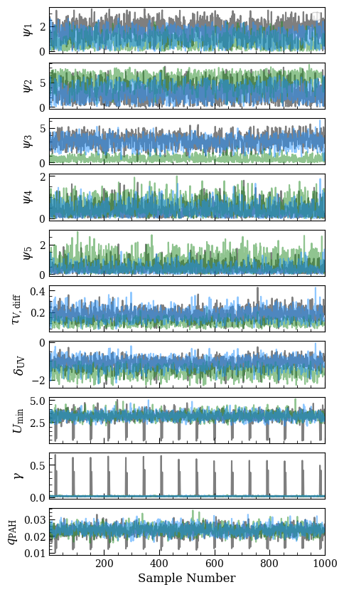
Where gray = PEGASE-Cloudy, blue = PEGASE, green = BPASS-Cloudy.
There’s not really a substantial difference except in the third bin of the SFH, which spans 100 Myr to 1 Gyr. The BPASS fit (pale green) puts much less star formation in that stellar age bin. We generally ascribe this to a red excess in the BPASS stellar spectra, which appears to be caused by overproduction of AGB stars, according to the 2018 BPASS release paper. We can overplot all the best-fit SED models and show the confidence regions on the SFHs, which will also make this clear:
[41]:
fig = plt.figure(figsize=(12,6))
ax1 = fig.add_axes([0.1, 0.26, 0.4, 0.64])
ax11 = fig.add_axes([0.2, 0.35, 0.2, 0.2])
ax2 = fig.add_axes([0.1, 0.1, 0.4, 0.15])
ax3 = fig.add_axes([0.56, 0.1, 0.34, 0.8])

fig, ax1 = lgh_pg_cl.sed_plot_bestfit(chain_pg_cl, logprob_chain_pg_cl,
                                   plot_components=False,
                                   ax=ax1,
                                   show_legend=False,
                                   total_kwargs={'color':'black', 'alpha':0.5})
fig, ax1 = lgh_pg.sed_plot_bestfit(chain_pg, logprob_chain_pg,
                                   plot_components=False,
                                   ax=ax1,
                                   show_legend=False,
                                   total_kwargs={'color':'dodgerblue', 'alpha':0.5},
                                   data_kwargs={'marker':'', 'linestyle':'', 'color':'none'})
fig, ax1 = lgh_bp_cl.sed_plot_bestfit(chain_bp_cl, logprob_chain_bp_cl,
                                   plot_components=False,
                                   ax=ax1,
                                   show_legend=False,
                                   total_kwargs={'color':'forestgreen', 'alpha':0.5},
                                   data_kwargs={'marker':'', 'linestyle':'', 'color':'none'})

fig, ax11 = lgh_pg_cl.sed_plot_bestfit(chain_pg_cl, logprob_chain_pg_cl,
                                   plot_components=False,
                                   ax=ax11,
                                   show_legend=False,
                                   total_kwargs={'color':'black', 'alpha':0.5})
fig, ax11 = lgh_pg.sed_plot_bestfit(chain_pg, logprob_chain_pg,
                                   plot_components=False,
                                   ax=ax11,
                                   show_legend=False,
                                   total_kwargs={'color':'dodgerblue', 'alpha':0.5},
                                   data_kwargs={'marker':'', 'linestyle':'', 'color':'none'})
fig, ax11 = lgh_bp_cl.sed_plot_bestfit(chain_bp_cl, logprob_chain_bp_cl,
                                   plot_components=False,
                                   ax=ax11,
                                   show_legend=False,
                                   total_kwargs={'color':'forestgreen', 'alpha':0.5},
                                   data_kwargs={'marker':'', 'linestyle':'', 'color':'none'})

ax11.set_xlim(0.1, 2)
ax11.set_ylim(5e8, 2e10)
ax1.set_xticklabels([])

fig, ax2 = lgh_pg_cl.sed_plot_delchi(chain_pg_cl, logprob_chain_pg_cl,
                                   ax=ax2,
                                   data_kwargs={'marker':'D', 'color':'k', 'markerfacecolor':'k', 'capsize':2, 'linestyle':'', 'alpha':0.5})
fig, ax2 = lgh_pg.sed_plot_delchi(chain_pg, logprob_chain_pg,
                                   ax=ax2,
                                   data_kwargs={'marker':'D', 'color':'dodgerblue', 'markerfacecolor':'dodgerblue', 'capsize':2, 'linestyle':'', 'alpha':0.5})
fig, ax2 = lgh_bp_cl.sed_plot_delchi(chain_bp_cl, logprob_chain_bp_cl,
                                   ax=ax2,
                                   data_kwargs={'marker':'D', 'color':'forestgreen', 'markerfacecolor':'forestgreen', 'capsize':2, 'linestyle':'', 'alpha':0.5})


fig, ax3 = lgh_pg_cl.sfh_plot(chain_pg_cl, ax=ax3,
                              shade_kwargs={'color':'k', 'alpha':0.3, 'zorder':0},
                              line_kwargs={'color':'k', 'zorder':1})
fig, ax3 = lgh_pg.sfh_plot(chain_pg, ax=ax3,
                           shade_kwargs={'color':'dodgerblue', 'alpha':0.3, 'zorder':0},
                           line_kwargs={'color':'dodgerblue', 'zorder':1})
fig, ax3 = lgh_bp_cl.sfh_plot(chain_bp_cl, ax=ax3,
                              shade_kwargs={'color':'forestgreen', 'alpha':0.3, 'zorder':0},
                              line_kwargs={'color':'forestgreen', 'zorder':1})
/Users/eqm5663/Research/code/plightning/lightning/stellar/pegase.py:1073: RuntimeWarning: divide by zero encountered in log10
  np.log10(np.transpose(self.Lnu_obs, axes=[1,2,0,3])),
/Users/eqm5663/miniconda3_arm64/envs/ciao-4.16/lib/python3.11/site-packages/scipy/interpolate/_rgi.py:418: RuntimeWarning: invalid value encountered in multiply
  term = np.asarray(self.values[edge_indices]) * weight[vslice]
/Users/eqm5663/Research/code/plightning/lightning/stellar/pegase.py:449: RuntimeWarning: divide by zero encountered in log10
  finterp = interp1d(self.Zmet, np.log10(self.Lnu_obs), axis=1)
/Users/eqm5663/miniconda3_arm64/envs/ciao-4.16/lib/python3.11/site-packages/scipy/interpolate/_interpolate.py:701: RuntimeWarning: invalid value encountered in subtract
  slope = (y_hi - y_lo) / (x_hi - x_lo)[:, None]

The color scheme is the same as above: gray = PEGASE-Cloudy, blue = PEGASE, green = BPASS-Cloudy.
The inset in the top panel blows up the optical-NIR portion of the SED to show differences between the models. The red excess from the BPASS models is clearly visible between 1-2 microns. Minimizing this excess leads to suppression of the third SFH bin and a slight enhancement of the second. We can look at the derived \(M_{\star}\) and SFR to see if this has a downstream effect:
[45]:
import corner

SFR100_pg_cl = 0.1 * chain_pg_cl[:,0] + 0.9 * chain_pg_cl[:,1]
SFR100_pg = 0.1 * chain_pg[:,0] + 0.9 * chain_pg[:,1]
SFR100_bp_cl = 0.1 * chain_bp_cl[:,0] + 0.9 * chain_bp_cl[:,1]

mstar_coeff_pg_cl = lgh_pg_cl.stars.get_mstar_coeff(chain_pg_cl[:,5])
mstar_coeff_pg = lgh_pg.stars.get_mstar_coeff(chain_pg[:,5])
mstar_coeff_bp_cl = lgh_bp_cl.stars.get_mstar_coeff(chain_bp_cl[:,5])

mstar_pg_cl = np.sum(mstar_coeff_pg_cl * chain_pg_cl[:,:5], axis=1)
mstar_pg = np.sum(mstar_coeff_pg * chain_pg[:,:5], axis=1)
mstar_bp_cl = np.sum(mstar_coeff_bp_cl * chain_bp_cl[:,:5], axis=1)

labels = [r'$\log M_{\star}~[\rm M_{\odot}]$', r'$\rm SFR_{100}~[\rm M_{\odot}~yr^{-1}]$']
fig = corner.corner(np.stack([np.log10(mstar_pg_cl), SFR100_pg_cl], axis=-1),
                    labels=labels,
                    smooth=1,
                    color='k')
fig = corner.corner(np.stack([np.log10(mstar_pg), SFR100_pg], axis=-1),
                    labels=labels,
                    smooth=1,
                    color='dodgerblue', fig=fig)
fig = corner.corner(np.stack([np.log10(mstar_bp_cl), SFR100_bp_cl], axis=-1),
                    labels=labels,
                    smooth=1,
                    color='forestgreen', fig=fig)
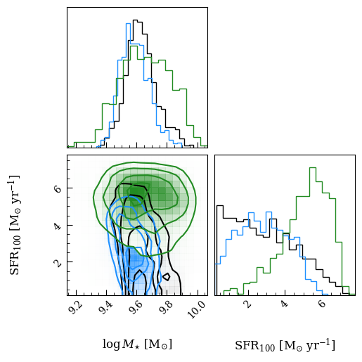
The stellar population differences don’t seem to create a strong bias in \(M_{\star}\). However, in this case, we see a slight difference in the SFRs, though they are statistically consistent. See the appendices in Lehmer+(2024) for a somewhat more robust comparison between SFR and stellar masses derived using PEGASE-Cloudy and BPASS-Cloudy models on a diverse sample of ~80 galaxies.
[ ]: